Numerical modeling of forest fire cycles and the role of topography

Following the 2011 Las Conchas fire in the Jemez Mountains, we have been studying the effects of wildfire on landscapes. In one numerical modeling and data analysis study, geomorphologists and fire scientists on the UA CZO team have been developing numerical models that integrate geomorphic properties into improved models of wildfire cycles.

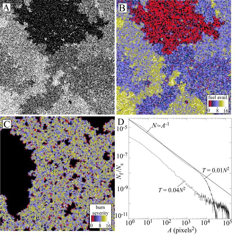
Fire scientists have long been interested in three important aspects of fire: 1) the frequency-size distributions of fires, which tend to follow a power law, 2) the spatial patterns of burn severity, and 3) the statistics of the patchy mosaic of forests left behind by many overlapping fire events. Figure 1 illustrates patterns in fire activity from a simple model of forest fires proposed by Malamud et al. (1998). During each time step of this model, a grid point is chosen at random and a tree is added to that grid point if one does not exist. Every T time steps, a spark is added to a random location and a fire burns that location (if a tree exists) and all adjacent locations in a connected cluster of sites with trees. This simple model gives a power law frequency-size distribution of fire events similar to that observed in real data.

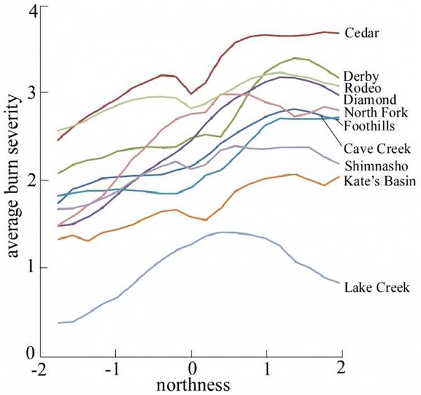
The Malamud et al. (1998) model has several unrealistic aspects. UA CZO scientists have shown that by including how topographic slope and aspect control the rate of fuel accumulation in forests, a more accurate model for forest fire cycles is obtained. Figure 2 shows the relationship between burn severity and topographic northness in 10 large recent forest fires of the western U.S. Northness is defined as the product of the sine of the slope and the cosine of the aspect. More north-facing slopes in water-limited landscapes of the western U.S. tend to have more fuel available to burn, and Figure 2 shows that they tend to burn hotter.

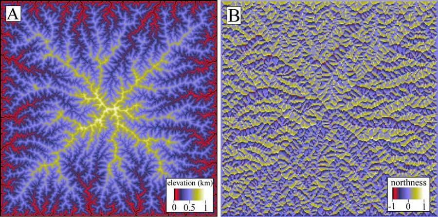
In the new model we developed, a landscape evolution model is used to create a fractal landscape (Fig. 3). The northness map from that landscape (Fig. 3B) is then used as input to a forest fire model that grows trees preferentially on north-facing slopes in a manner consistent with the results of Figure 2.

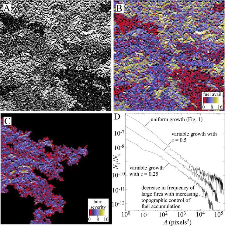
Figure 4 illustrates results from our forest fire model that includes the effects of topography on fuel accumulation rates. This model simultaneously reproduces the same patterns in real fires and fire-affected forests with respect to 1) the frequency-size distribution of fires (with a rolloff in the frequency of large fires below the power-law distribution), 2) the spatial variations in burn severity, and 3) the spatial variations in available fuel.

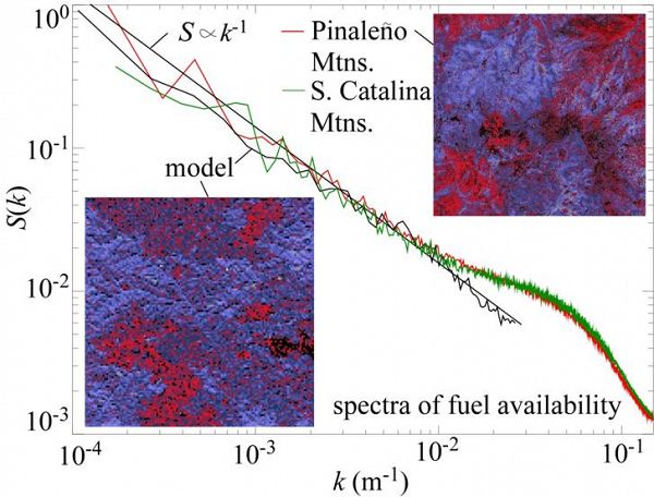
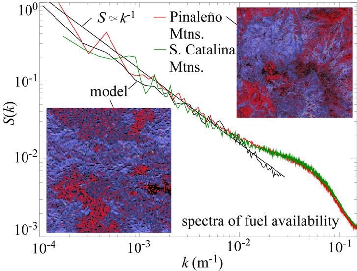
In the new model, burn severity and fuel availability in forests both have a fractal spatial structure known as 1/f noise (Fig. 5). In a 1/f noise, the power spectrum of spatial variations is inversely proportional to the wave number k. As Figure 5 shows, the power spectrum of fuel in real fire affected forests in the Pinaleno and Santa Catalina Mountains near Tucson (as measured by airborne lidar) are 1/f noises. The model reproduces the same trend as the observed spectra over spatial scales of 100 m to approximately 10 km.

Quantifying extreme post-fire landscape response in the Jemez River basin, New Mexico

The Jemez River basin (location of the University of Arizona CZO project) was recently the site of the largest wildfire in New Mexico state history. This event presents a unique opportunity to quantify and understand the geomorphic, hydrologic, and ecological response to a major perturbation using high-resolution mapping, field measurement/data collection, and numerical modeling.

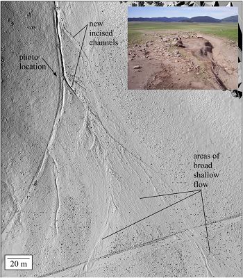
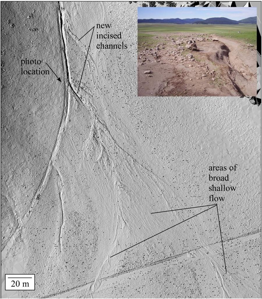
Figure 6 illustrates an example of the extreme geomorphic response following the Las Conchas fire (630 km² burned) and subsequent rainfall events of the 2011 monsoon season. Prior to the fire, this piedmont had no active channels and was entirely grass-covered. A single thunderstorm on August 5, 2011 formed a 1 km-long gravel-dominated distributary-channel system that transported boulders up to 1 m in diameter (see inset photo). In the weeks following the fire, we documented similar extreme erosion and deposition in 5 fire-affected drainage basins. Interestingly, much of the sediment removed from the steep hillslopes of fire-affected drainage basins is not being transported to piedmonts like that illustrated in Figure 6. In the tributary drainage basins upstream from many piedmonts, we have observed deposition and channel avulsions at many tributary junctions, suggesting that the sediment deposited on the piedmont represents only a fraction of the total sediment being removed from hillslopes (the rest is stored at multiple places within the basin). A spatially-complete map of erosion/deposition is needed to properly quantify the sediment budget and geomorphic change caused by the fire and the subsequent monsoon rainfall events. To obtain that map NCALM will be flying post-fire lidar in May, 2012.

A key goal of hillslope/fluvial geomorphology is to predict the geomorphic response (i.e. erosion and deposition) of landscapes using input data for initial landscape morphology, soil properties, vegetation cover, and rainfall for one or more events. Numerical models exists that can predict such changes, but these models suffer from a lack of high-resolution, spatially-distributed data for test cases (National Academy of Sciences, 2009). The geomorphic modeling community has identified the acquisition of high-resolution, spatially-distributed data for landscape response to major perturbations as a high priority (CSDMS Working Group, 2004).

The airborne LiDAR data and resulting geomorphic change map is just one piece of our larger goal to construct a database usable by hydrologic and landscape evolution modelers worldwide to test the ability of their models to predict the landscape response to a major perturbation. We will derive hourly spatially-distributed rainfall data for the 2011 monsoon season using the 5 rain gages currently operating in the fire-affected areas of the Jemez River basin. These rain gages will be combined with NEXRAD radar data to provide spatially-complete maps of rainfall at 1 hour intervals. The pre- and post-fire LiDAR data will be processed to provide canopy height, biomass, and burn severity datasets for pre- and post-fire conditions. Infiltration measurements collected by the CZO team during the 2011 monsoon season in areas of low, moderate, and severe burn intensities (in addition to measurements in non-fire-affected areas) will be used to infer values of soil permeability and their relationship to burn severity.

What we will do with the airborne LiDAR data and complimentary datasets:

1) Mapping burn severity

A burn severity map has been produced for the Las Conchas fire based on differences between pre- and post-fire AVHRR NDVI greenness values. These maps provide a measure of fire intensity but field observations by the UA CZO team and VCNP staff have identified many areas where the map is not accurate. LiDAR data will provide a more detailed and accurate index of fire severity. LiDAR allows us to quantify the living and dead vegetation (fuel) changes that are a direct consequence of the fire at high resolution. Pre-post differences will provide one of the highest spatial resolution assessments of vegetation/fuel impacts of wildfire at landscape scales ever obtained. Pilot data from another UA study indicates 95% accuracy (n = 398 trees) at discriminating living vs. dead conifers (Swetnam, T.L., doctoral dissertation, in prep.) using airborne LiDAR.

2) Mapping erosion/deposition caused by the 2011 monsoon season

We will difference the 2010 and 2012 LiDAR products to obtain a map of erosion and deposition for the fire-affected area. Nominally, NCALM provides 1 m/pixel bare-earth raster layers but we anticipate using the raw LiDAR point cloud data to optimize our geomorphic change detection maps (i.e. optimal algorithms will likely differ among areas with and without large woody vegetation) and provide the highest resolution possible. Differencing of LiDAR products must be done with care due to potential errors/uncertainties in absolute GPS control, so it may be necessary to use fixed structures (e.g. edges of buildings) to post-process the NCALM data for optimal accuracy. In areas of sediment deposition, the thickness of sediment deposited above the buried grass layer provides ground truth measurements that can be used to validate the LiDAR-derived measures of erosion/deposition. We will measure depositional thicknesses at several hundred locations, surveyed with differential GPS, during the 2012 LiDAR flight for this purpose.

3) Mapping surface changes that indicate surface flow without significant erosion/deposition

In the field we have observed locations where the erosion/deposition was relatively small (i.e. < 5 cm) but significant flow nonetheless occurred during recent monsoon storms as evidenced by thin layers of deposited clastic or organic material and/or disturbance of grasses. Such areas are important to include/resolve in our mapping because they provide indicators of water flow necessary to validate hydraulic models even though relatively little geomorphic change is occurring in those areas. We will use a combination of LiDAR intensity and small-scale roughness to classify areas where the amount of erosion/deposition was too small to be resolved by differencing of airborne LiDAR datasets but where flow nonetheless occurred. These activities will result in a methods-based journal article on how best to use airborne and ground-based LiDAR to infer flow depths and velocities (based on the texture of material transported) following major flood events.

4) Perform regression analyses to quantify hillslope sediment yield and how it varies with slope, drainage area, burn intensity, and rainfall intensity/duration

A key goal of our work is to derive empirical expressions for how sediment yield varies as a function of slope, drainage area, burn intensity, and rainfall intensity/duration in post-fire environments. Our working hypothesis is that sediment yield will increase nonlinearly with slope, burn intensity, and rainfall intensity/duration and will decrease nonlinearly with drainage area. How sediment yield varies with burn intensity is not well constrained given the fact that sediment yield has never been measured for enough fire-affected drainage basins of varying burn intensity to calibrate such a curve. This will be the first study with enough data to calibrate such a relationship.

5) Continued acquisition of ground-based LiDAR over time in select areas

We will continue to acquire terrestrial laser scans (ground-based LiDAR) similar to that in Figure 1 in selected areas over time in order to quantify how sediment yields change through time as the landscape "recovers." Conceptual models for the landscape adjustment to fire predict that landscapes return to a state similar to pre-burn conditions following an exponential decrease from an initial post-fire peak to a new quasi-equilibrium condition over a time scale of several years to decades. Our CZO project aims to calibrate that recovery graph and its ecologic, hydrologic, and geomorphic controls. Ground-based LiDAR will play an important role in that effort but it is important to emphasize that ground-based LiDAR cannot possibly measure geomorphic change in even a fraction of the total fire-affected area. As such, airborne LiDAR data is needed.