Seeing the subsurface with a sledgehammer instead of a shovel
Brady Flinchum in Adventures in the Critical Zone

Mar 21, 2017
Do you know where plants get water during the long summer months when the region has not had any rain or snow for weeks? Have you ever wondered how the soil that you walk on was formed? Have you ever questioned how much water a groundwater aquifer can hold and how much water actually recharges the aquifer? These are increasingly important questions that need to be answered so that we can predict how the Earth’s systems will respond to changing climactic conditions—and yet these questions are extremely complex, interdisciplinary, and difficult to answer because the subsurface is inaccessible on large spatial scales. My name is Brady Flinchum, I am a near-surface geophysicist at the University of Wyoming.
Much like a doctor uses an x-ray to see inside the human body, I utilize geophysical tools to image the current subsurface structure over large areas. The subsurface architecture of the critical zone can reveal the processes that regulate water movement, the rate at which rock is transformed into soil, and the water availability for plants. In the following blog post, I will explain some of the advantages and drawbacks of using near-surface geophysical methods to image the subsurface and show that the critical zone varies in thickness and structure across the United States, much like the various ecosystems and plants that inhabit the surface.

Figure 1. The route that the Wyoming Center for Environmental Hydrology and Geophysics (WyCEHG) team took in the summer of 2015 to collect geophysical data at five different sites in five different states. Three of the five sites were critical zone observatories. The site locations are marked by yellows stars.
During the summer of 2015, I was lucky enough to be part of a team that traveled to five different sites in five different states (Figure 1). We encountered diverse landscapes and ecosystems ranging from the flat plains east of the Front Range to endless mountains of the Great Basin and the beautiful deserts of Arizona to the mighty Sequoia trees in the Southern Sierra’s. So how does the critical zone structure vary at all five of these sites? Although I work with many geophysical tools, I will focus on a technique called shallow seismic refraction.
To collect shallow seismic refraction data, it requires a small team because of the hundreds of pounds of gear that we have to lay out in a straight line over rugged terrain. We plant geophones into the ground with a small metal spike (Figure 2a). The geophones measure the vertical movement of the ground and they are so sensitive you can see the vibrations from a person sneezing if they were standing nearby. We use anywhere from 24 to 240 individual geophones per survey. All of the geophones are connected to a seismograph through long cables. The seismographs digitize the ground motion and send it to the computer. To power the system we have to distribute up to nine 80 lb car batteries along the profile, which can be physically exhausting.
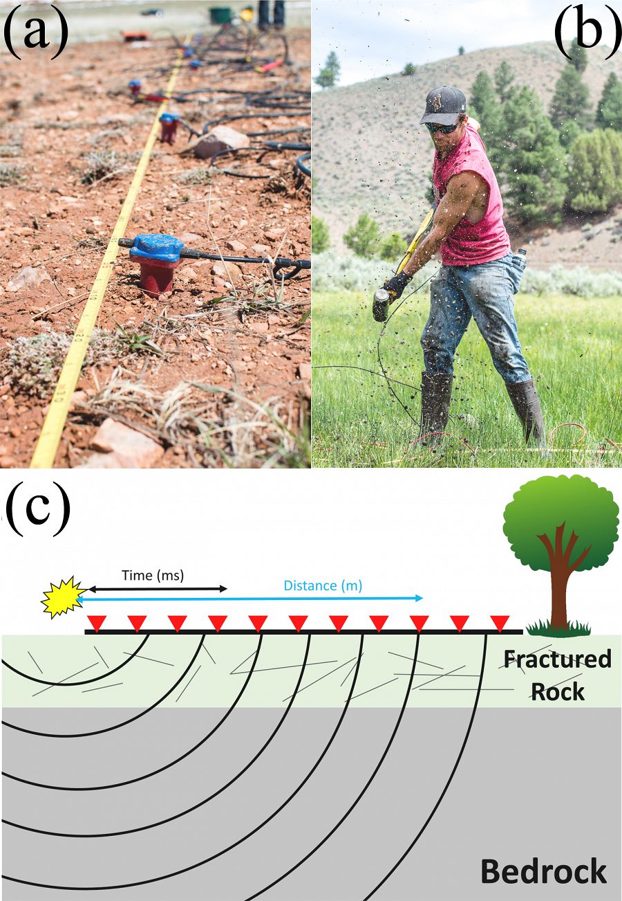
Figure 2. The basics of collecting shallow seismic refraction data are shown. (a) Geophone planted into the ground. (b) Matt Elliot swinging the sledgehammer at the site in Oregon. (c) A basic cartoon demonstrating how energy travels from source to receiver. We measure how long it takes from the source (yellow explosion) to each geophone (red triangles).
Once all of the equipment is laid out—we get to make noise! We use a sledgehammer as the seismic source, no matter if we are surveying solid rock or a swamp (Figure 2b). The general idea behind a seismic refraction survey is to hit the ground really hard and then measure how the energy travels through the Earth. As energy travels from the source to the receivers we can measure the arrival of the energy with an accuracy of a few milliseconds (Figure 2c). Since we know the distance from source to each receiver we can calculate an apparent velocity, which is just distance over time. Although there is more complicated physics that govern how the wave field travels through the subsurface, we understand the physics well enough to construct a two dimensional velocity model. The resulting velocity model is essentially our best guess of the subsurface velocity structure.
So how is the seismic velocity related to critical zone structure? Well the answer is that seismic energy travels at different speeds through different materials. If you have a solid competent piece of granite, the seismic velocity is between 4000 and 5000 m/s, but softer more friable material has seismic velocities on the order of 300 – 700 m/s. Using shallow seismic refraction allows us to differentiate between solid rock and soft material. Of course solid rock will likely hold a small amount of water, whereas the soft friable material could potentially hold a lot of water and be where plants are drawing their water during the dry months. So one of biggest advantages of geophysical methods is their ability to measure geophysical parameters, like seismic velocities, over large spatial scales. Of course all methods have a trade-off. To improve our models of critical zone processes, we actually want to know the fracture density, water holding capacity, or the chemistry of the material. We know that seismic velocities are linked to these properties of interest but they still have to be interpreted using other supporting data sets. This ambiguity is one of the draw backs to geophysical methods and why I work with an interdisciplinary team of scientists to interpret the geophysical data.
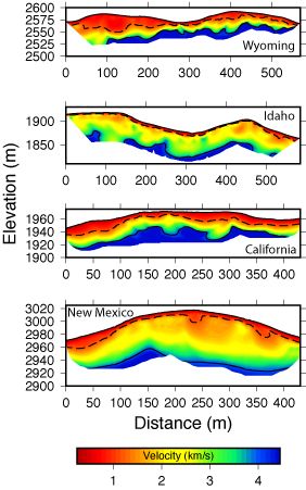
Figure 3. Seismic velocity results for four of the five sites shown in Figure 1. All of the profiles are plotted at 3x vertical exaggeration and on the same color scale. The dotted line represents a velocity of 1.2 km/s and the solid line is 4.0 km/s. Each of these lines are just a small subset of the data that we collect during the week and just these four lines alone cover approximately 1.8 km (~20 football fields!).
From our geophysical observations we collected over the summer of 2015, our data shows, to no surprise, that the subsurface structure at the five sites is diverse. The seismic velocity sections from each of the five sites are shown in Figure 3 and are all plotted on the same velocity scale. To a first order, you can interpret these images as slower velocities representing more weathered and friable material and faster velocities being more representative of the underlying bedrock. Keep in mind, myself and many others are still researching exactly what these velocities mean in terms of weathering indices, porosity, fractured density, and critical zone structure. But the most exciting part about these data is that we collected the same data set on five different sites. Collecting the same types of data sets over different landscapes will allow us to isolate variables that regulate critical zone structure such as: lithology, climate, or position on the landscape (i.e. valley bottom or ridge top). As we continue to improve our understanding of the relationships between geophysical, hydrologic and geochemical parameters we will gain better understanding of the complex region of Earth’s subsurface we call the critical zone and make progress to understanding Earth’s systems.
Figure 1. The route that the Wyoming Center for Environmental Hydrology and Geophysics (WyCEHG) team took in the summer of 2015 to collect geophysical data at five different sites in five different states. Three of the five sites were critical zone observatories. The site locations are marked by yellows stars.
Figure 2. The basics of collecting shallow seismic refraction data are shown. (a) Geophone planted into the ground. (b) Matt Elliot swinging the sledgehammer at the site in Oregon. (c) A basic cartoon demonstrating how energy travels from source to receiver. We measure how long it takes from the source (yellow explosion) to each geophone (red triangles).
Figure 3. Seismic velocity results for four of the five sites shown in Figure 1. All of the profiles are plotted at 3x vertical exaggeration and on the same color scale. The dotted line represents a velocity of 1.2 km/s and the solid line is 4.0 km/s. Each of these lines are just a small subset of the data that we collect during the week and just these four lines alone cover approximately 1.8 km (~20 football fields!).
Guest Author

Brady Flinchum
CZO COLLABORATOR, GRAD STUDENT. . Specialty: Near-Surface Geophysics
Geophysics Outreach / Education Research EDUCATION/OUTREACH General Public
COMMENT ON "Adventures in the Critical Zone"
All comments are moderated. If you want to comment without logging in, select either the "Start/Join the discussion" box or a "Reply" link, then "Name", and finally, "I'd rather post as a guest" checkbox.
ABOUT THIS BLOG

ABOUT THIS BLOG
Justin Richardson and his guests answer questions about the Critical Zone, synthesize CZ research, and meet folks working at the CZ observatories
General Disclaimer: Any opinions, findings, conclusions or recommendations presented in the above blog post are only those of the blog author and do not necessarily reflect the views of the U.S. CZO National Program or the National Science Foundation. For official information about NSF, visit www.nsf.gov.
Explore Further